Simple Heat Transfer Tutorial
This tutorial provides an introduction to running simulations with Serac and demonstrates the setup of a simple steady-state heat transfer problem.
The full source code for this tutorial is available in examples/conduction/simple_conduction.cpp, =
which demonstrates C++ configuration of a heat transfer physics module.
The heat transfer modeled in this section is based on the formulation discussed in Heat Transfer.
Setting Up Includes and Initializing
Serac provides a single unified header for all classes and functions needed by users. Shown here:
#include "serac/serac.hpp"
Note
If you are concerned about compile times, you may use the individual headers, but for this example we encourage you to use the single header which will bring in all you need.
We're now ready to start our main() function. Serac's ApplicationManager class automatically,
through RAII, initializes and finalizes much of the boilerplate setup required for each simulation,
e.g., MPI, logging. All you need to do is instantiate the class before other Serac functionality:
int main(int argc, char* argv[])
{
  // Initialize and automatically finalize MPI and other libraries
  serac::ApplicationManager applicationManager(argc, argv);
Warning
Since Serac's initialization helper initializes MPI, you should not call MPI_Init directly.
To simplify saving to an output file and restarting a simulation, Serac stores critical state information, like
the mesh, fields, and individual finite element states, in a single StateManager object.
  axom::sidre::DataStore datastore;
  serac::StateManager::initialize(datastore, "without_input_file_example");
Constructing the Mesh
Serac's mesh utilities include support for reading meshes from a file and for generating meshes of common solids,
like cuboids, rectangles, disks, and cylinders. In this introductory example, we will use a simple square
mesh with 10 quadrilateral elements in each space dimension for 100 elements total. Serac's mesh class,
serac::Mesh, takes in one of these meshes and automatically adds it to the StateManager. Once created, the
primary mesh will be registered with the StateManager:
  std::string mesh_tag{"mesh"};
  auto mesh = std::make_shared<serac::Mesh>(serac::buildRectangleMesh(10, 10), mesh_tag);
After constructing the serial mesh, we call refineAndDistribute to distribute it into a parallel mesh.
Constructing the Physics Module
The most important parts of Serac are its physics modules, each of which corresponds to a particular discretization
of a partial differential equation (e.g., continuous Galerkin finite element method for heat transfer).
In this example, we are building a heat transfer simulation, so we include Serac's HeatTransfer module and
thermal material models:
  // Create a Heat Transfer class instance with Order 1 and Dimensions of 2
  constexpr int order = 1;
  constexpr int dim = 2;

  serac::HeatTransfer<order, dim> heat_transfer(serac::heat_transfer::default_nonlinear_options,
                                                serac::heat_transfer::default_linear_options,
                                                serac::heat_transfer::default_static_options, "thermal_solver", mesh);
When using the C++ API, the HeatTransfer constructor requires the polynomial order of the elements and
the dimension of the mesh at compile time, i.e. they are template parameters. We also need to pass the options
for solving the nonlinear system of equations and ordinary differential equations arising from the
discretization. In this example, we use the default static heat transfer options.
Configuring Material Conductivity
We define a material model that includes information needed for the constitutive response needed by the physics solver.
In this example, we define a linear isotropic conductor with uniform density, heat capacity, and conductivity (kappa).
That material model is then passed to the HeatTransfer object. Note that this material model could be user-defined.
  constexpr double kappa = 0.5;
  serac::heat_transfer::LinearIsotropicConductor mat(1.0, 1.0, kappa);

  heat_transfer.setMaterial(mat, mesh->entireBody());
Setting Thermal (Dirichlet) Boundary Conditions
The following snippets add two Dirichlet boundary conditions:
One that constrains the temperature to 1.0 at boundary attribute 1, which for this mesh corresponds to the side of the square mesh along the x-axis, i.e., the "bottom" of the mesh.
One that constrains the temperature to \(x^2 + y - 1\) at boundary attributes 2 and 3, which for this mesh correspond to the right side and top of the mesh, respectively.
  const std::set<int> boundary_constant_attributes = {1};
  constexpr double boundary_constant = 1.0;

  auto ebc_func = [boundary_constant](const auto&, auto) { return boundary_constant; };
  heat_transfer.setTemperatureBCs(boundary_constant_attributes, ebc_func);

  const std::set<int> boundary_function_attributes = {2, 3};
  auto boundary_function_coef = [](const auto& vec, auto) { return vec[0] * vec[0] + vec[1] - 1; };
  heat_transfer.setTemperatureBCs(boundary_function_attributes, boundary_function_coef);
Running the Simulation
Now that we've configured the HeatTransfer instance using a few of its configuration
options, we're ready to run the simulation. We call completeSetup to "finalize" the simulation
configuration, and then save off the initial state of the simulation. This also allocates and builds
all of the internal finite element data structures.
We can then perform the steady-state solve and save the end result:
  heat_transfer.completeSetup();
  heat_transfer.outputStateToDisk();

  heat_transfer.advanceTimestep(1.0);
  heat_transfer.outputStateToDisk();
Note
The dt variable does not actually get used in this quasistatic simulation.
This should produce the following initial state:
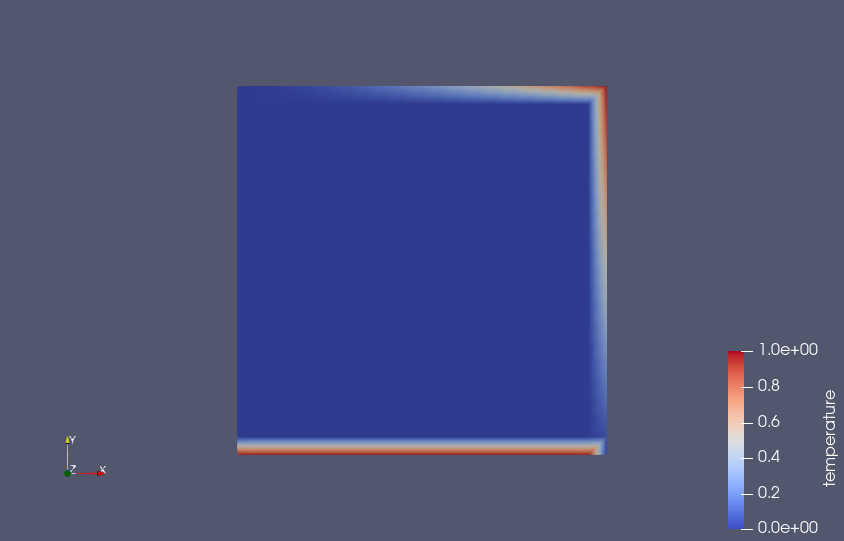
Note the areas of the mesh where the boundary conditions were applied.
The final (steady-state) solution should look like the following:
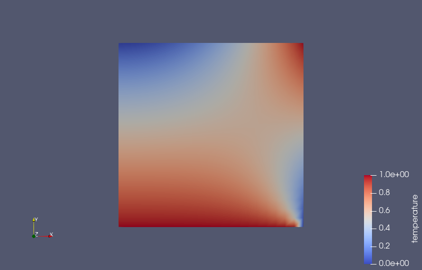
The end result is not particularly impressive, but should be fairly intuitive.
Cleaning Up
Serac's ApplicationManager class will automatically finalize it's previously mentioned initialized classes
through RAII when it falls out of scope. To end your simulation simply return from the main like any
other C++ program:
  return 0;
}